On this page we have put together a glossary of biosensors terms that are useful for Biosensor Developers. This page is intended to help guide conversations with clients and collaborators when discussing biosensors and biosensor specifications, at the time of writing it is also our intention to implement the calculations of such parameters into Djuli, our Cloud Electrochemical Biosensor Database.

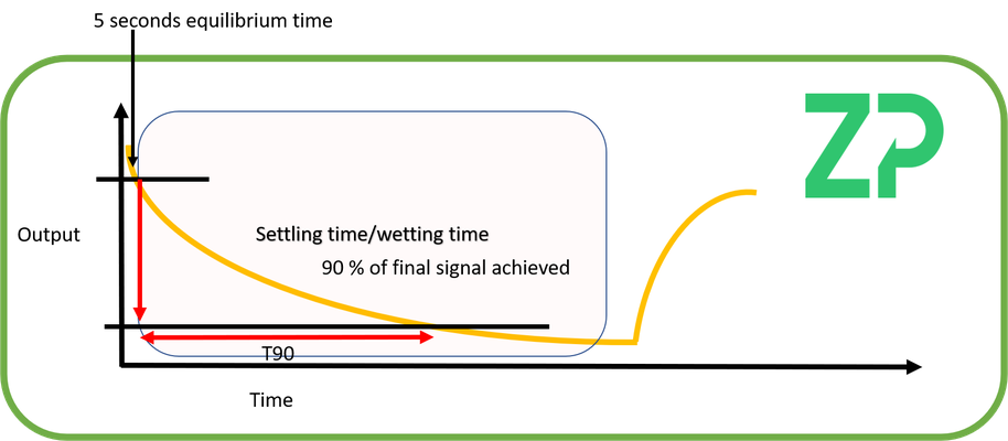
Settling time - At ZP we sometimes refer to this as wetting time, but here we will  say the settling time is the time it takes for the sensor to reach a stable output after first being activated.

There is no universal definition as to 'stable output' and can be client and application specific, but the time taken to reach within 10 % of the final value is a good starting definition.

A procedure for measuring the settling time for an amperometric biosensor is to:

1) Activate the electrode at the required voltage for 5 seconds.

2) Start the data logging after the initial 5 seconds of equilibrium.

3) Measure the time it takes for the signal to have reached within 10 % of the final value, which we define at ST90 (settling time 90 %).

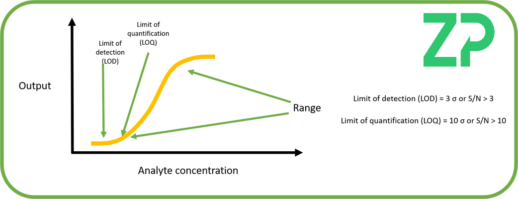
Biosensor Analytical Range - The analytical range of a biosensor is the interval between the upper and lower concentrations where the sensor has been demonstrated to be precise. The lower end of the range can be defined both by the Limit of Detection (LoD) and the Limit of Quantification (LoQ). 

Limit of Detection (LoD)

The Limit of Detection  is defined as when the signal (S) is three times greater than the noise > S/N, another another form of the same statement is that the signal is detectable when the signal is greater than three standard deviations, S > 3 x std.

Limit of Detection (LoQ)

The Limit of Quantification  is defined as when the signal (S) is ten times greater than the noise > S/N, another another form of the same statement is that the signal is detectable when the signal is greater than ten times the standard deviations, S > 10 x std.

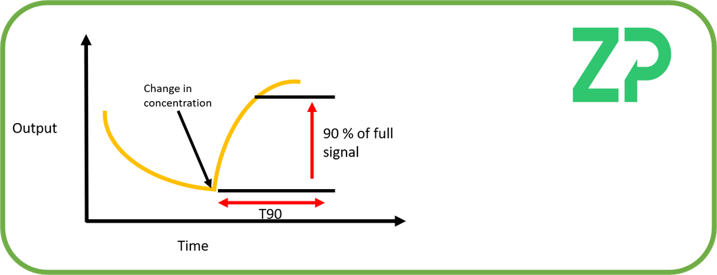
Biosensor response time

The biosensor response time is the time it takes for the sensor output to reach it's new signal after being exposed to a change in analyte concentration, this is often quoted as T90, which is the time it takes for the signal to reach 90 % of its final value.

Signal Resolution

There is a confusion when talking about resolution of biosensors, as there are at least two sub-divisions: signal resolution and electronics resolution.

On this page we will focus on signal resolution. The ability of a signal to resolve or have a signal  output that is discernible between two concentrations is really a function of the system or experimental setup. In the case of an amperometric electrochemical biosensor the ability to resolve one analyte concentration from another analyte concentration is dependent on the experimental noise, where the source of this noise includes: magnetic stirrers, pulsed flow, turbulent flow, electromagnetic, mains electricity noise, etc.

Electrochemical biosensors can detect in the femto molar and pico molar concentrations but to do so requires well designed test conditions and experimental setup, but two resolve an output between two concentrations the change in signal should be equal or greater than 3 x standard deviations.

Clinical Range - The range of analyte concentration in which a biosensor would be expected to operate. For example blood glucose levels can be between 1 mM to 20 mM (18 mg/dL to  360 mg/dL)

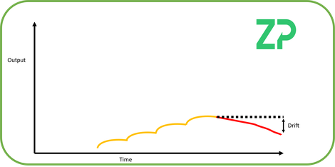
Signal Drift -  Signal drift describes the stability of a sensor's output signal in a situation where all conditions are fixed. When all conditions are fixed then the sensor should give a stable signal output; a temperature sensor is an example of a sensor/transducer type where the signal output is often  stable, but with many chemical and biological sensors the signal may not be stable and is described as drifting with time, for example most laboratory pH sensors are calibrated at least daily because of the inherent drift in these types of sensors. The drift over time can be used to calculate the rate of drift.

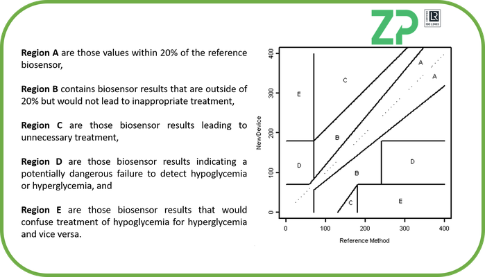
Error Grid Analysis (EGA) - The accuracy that a biosensor requires at any specific analyte concentrations is linked to the consequences that a false reading would have on the patient. For example in the Clarke Error Grid for blood glucose meters (BGM) it is only within zone A that the BGM has to be within 20 % of the reference value.

When you look at zone A it has a shape that reflect that the sensor needs to be most accurate at < 90 mg/dL, this is because this is indicative of a hypoglycemic region and so an untreated patient in this region could go into coma and die. Similarly when you look at Region B you can see that the sensor can be in inaccurate but this does not have a clinical impact and so is acceptable. When designing a biosensor system and describing the necessary accuracy then one has to think about accuracy in terms of whether inaccuracy will cause the patient harm or cause an incorrect clinical intervention.

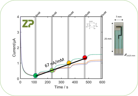
Biosensor Sensitivity 

 Biosensor Sensitivity is the change in signal per change in concentration. In the adjacent image we have calculated the linear sensitivity for a glucose sensor, which is approximately 67 nA/mM.

Biosensor Specificity versus Biosensor Selectivity

The terms specificity and selectivity are wrongly interchanged when describing biosensors; an important difference between the terms  is that specificity is the ability to assess an exact analyte in a mixture, whereas selectivity is the ability to differentiate analytes in a mixture from each other.

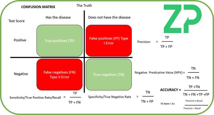
Confusion Matrix

The Confusion Matrix appears in many disciplines where categorizing a state as TRUE or FALSE is important, including medical diagnosis where answering questions such as 'does the patient have or not have COVID-19' is the question answered in part by the diagnostic. 

In these types of  application then a confusion matrix is very useful to calculate sensitivity, specificity, precision and accuracy of the medical diagnostic.

Receiver operating characteristic (ROC)

The ROC curve is related to the binary classifier  as described in the Confusion Matrix above.

As the threshold that separates disease from no disease is changed the true positive rate  and false positive  rate also changes, and this can be displayed in a ROC curve

For a well designed medical diagnostic then the population of values corresponding to disease and no disease sample are well separated and so for all threshold values the true positive rate is high and the area under the curve (AUC) is close to 1.0.

In a medical diagnostic where the values from no disease and disease samples start to overlap then the true positive rate is decreased and the AUC decreases.

A 'useless' medical diagnostic is one where the population of vales for disease and no disease samples are on top of each other and the subsequent ROC curve has AUC is close to 0.5, indicating that the diagnostic is no better than guessing.